Automatic License Plate Detection and Number Display

OVERVIEW :

Object Detection has become a key area, in the field of Artificial Intelligence(AI) and Machine Learning(ML). Along with Object detection and object recognition there is an area where you need to recognize the Content within the object detected or recognized.

This area has a lot of applications for example vehicle number plate detection, scanning the bar code and get the details, take photos of large shipping containers and get the required plate information, or license details, etc.

In this case study we will focus more on Automatic License plate detection and displaying the vehicle number present in it.

BUSINESS PROBLEM :

The Business problems we can try and solve are many. A few of them are.

1. Parking assistance or Vigilance systems — here in the parking lot(commercial, apartment) we can track every single vehicles time in , time out which helps in removing the manual effort.

2. Automated Toll gates — here as the vehicle approaches, the license number is detected and the respective details are fetched and allows the vehicle to pass through which removes the manual effort.

3. Vehicle Surveillance System - here you can track the traffic violators, and rash drivers vehicle details. Later send the candidate his respective ticket for the violations being made.

4. Manufacturing and Logistics Area - As there are more than a million shipping containers across the world, they need proper tracking, for the sake of goods delivery and mishaps. The License plate detection can be extended for it as well.

BREAKING IT DOWN TO MACHINE LEARNING PROBLEM:

In this article we will discuss how a machine learning model will help in detecting the number plate and extracting the information from the plate.

TABLE OF CONTENTS

1. Data description and Architectural approach

2. EDA

3. Splitting the data and building configuration scripts for Model Training

4. Validating the model with Sample Test Images

5. Improving the Model using YOLO v5

6. Metrics Evaluation

7. Model Deployment and Execution using Web App

8. Validating the YOLO model with Sample Demo and Test Images

9. Future enhancements and References

1. Data description and Architectural approach

The Train data is of 296 Images and its respective annotated Files. The Test data is of 80 Images and its respective annotated Files. Each of the image might contain multiple vehicles containing license plates, or a single vehicle with a license plate or just an image without any vehicle.

Architectural Approach:

Architectural Approach

STEP 1: Collecting the images from Internet and any other sources.

STEP 2: Once collected the images from web, we will save them into a folder. For the annotation purpose, I have used the tool ‘labelImg’ which you can find in the GITHUB link below:

GitHub - heartexlabs/labelImg: LabelImg is now part of the Label Studio community. The popular…

labelImg is a widely used open-source graphical annotation tool. It is only suitable for object localization or detection tasks, and it’s solely able to create rectangle boxes around considered objects.

Another advantage is that you can save/load annotations in 3 popular annotation formats: PASCAL VOC, YOLO.

Once the LableImg is installed, below figure shows the different options it has. As you can see we can select a directory and have all the images stored, and left and right arrow in the tool help in navigating through all the images.

Here we are creating a Rectangular box as that what we need to annotate and name it as a ‘number_plate’ Label.

LabelImg Tool used for Image Annotation or Labeling

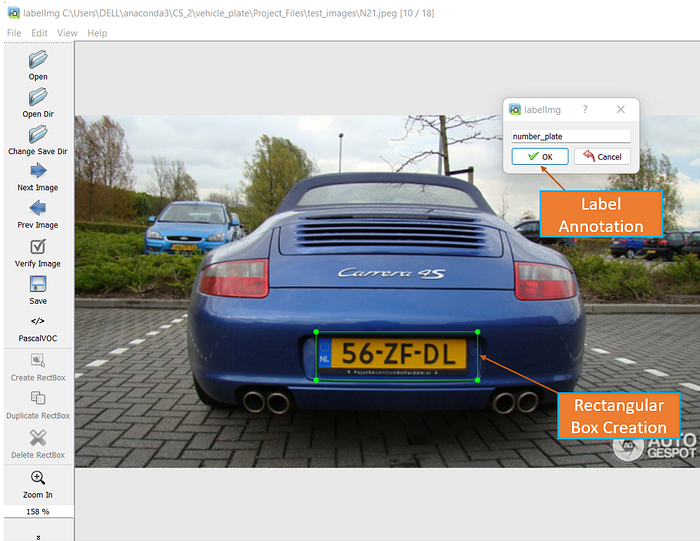
Once the box is drawn, we can save it as an XML file.

Image Annotation saved as XML

Sample Image file annotation with XML file as its output is show below.

Sample XML output of LabelImg Tool

STEP 3: After the annotation, we perform Data Pre-Processing, which include — reading every file and extracting the important elements from each file which can be used for Modeling purpose. We parse the XML and finally load it to a DataFrame for our Training and configuration needs.

Figure below shows, a dataframe after extracting important elements from XML.

DataFrame after extracting important elements from XML

STEP 4: In this step we train the model using the basic InceptionResNetV2, and extract the License plate.

STEP 5: Here we use that License plate detection image(ROI-Region Of Interest) and extract the text using Tesseract.

STEP 6: This whole project is done using a Web App via Python Flask Framework.

2 . Exploratory Data Analysis

Before going to any kind of modelling, we will always want to have a look at the kind of data that we have.

Now lets go ahead and check the data we have in pandas dataframe.

we can create a small utility function which will help in reading the files and get the required output, for example, given a filename(XML) with its path, it should produce the file path of the image(JPEG) with its name.

We can validate the Annotated Image and see how it looks like using the below code snippet.

file_path='\images\N101.jpeg'
img = cv2.imread(file_path)
cv2.rectangle(img,(134,312),(301,350),(34,119,255),3)
cv2.namedWindow('vehicle_plate',cv2.WINDOW_NORMAL)
cv2.imshow('vehicle_plate',img)
cv2.waitKey(0)
cv2.destroyAllWindows()

Rectangular Box showcasing number plate

Lets perform a small statistical analysis using x_max, xmin, y_max, and y_min by calculating the length and breadth of the rectangles.

Lets see the data distribution of length and breadth

#Create a distribution plot for x_length
sns.distplot(df.x_length,bins=20, color="g")
plt.title("Distribution of x_length", fontsize=20, color = 'green')
plt.show()

Distribution of Length and Breadth of the rectangle

From the above we can infer that length values range from 75 to 500 approx., and breadth values range from 30 to 200 approx. This is how it is distributed.

3 . Splitting the data and building configuration scripts for Model Training

Now that we have finished an initial level of analysis, lets do some pre-processing and build the script for Training purpose.

A. Firstly, we know that we need to predict the bounding box coordinates. Which means there will be 4 outputs (xmin,xmax,ymin,ymax)which will be part of Label.

B. Secondly we will build a list containing all the image paths for the iteration purpose and Pre-Processing purpose.

# Utility Function which gives image_path for a given File path as an input
def getFilename(filename):
    filename_image = xet.parse(filename).getroot().find('filename').text
    filepath_image = os.path.join('/images/',filename_image)
    return filepath_image

# List of Image Paths from DataFrame
image_path = list(df['filepath'].apply(getFilename))
image_path 

C. Thirdly, we would need to iterate through this Image path list.

Here we perform the following steps for Normalization of Input and Output:

1. we read every image and get the 3D shape of it
2. we convert it to a size (224,224) as we are using it for training on InceptionResNetV2 Model
3. We convert it to Array, and perform the Normalization Logic by dividing the values with 255 and store in data(input) list.
4. For the Labels Normalization, we collect the Labels[4 columns info], and we divide xmin/w, xmax/w, ymin/h, and ymax/h
5. This value we store in output array list

data = []
output = []
for ind in range(len(image_path)):
    image = image_path[ind]
    img_arr = cv2.imread(image)
    h,w,d = img_arr.shape
    # prepprocesing and Normalization of Input
    load_image = load_img(image,target_size=(224,224))
    load_image_arr = img_to_array(load_image)
    norm_load_image_arr = load_image_arr/255.0 # normalization
    # normalization to labels/output
    xmin,xmax,ymin,ymax = labels[ind]
    nxmin,nxmax = xmin/w,xmax/w
    nymin,nymax = ymin/h,ymax/h
    label_norm = (nxmin,nxmax,nymin,nymax) # normalized output
    # -------------- append
    data.append(norm_load_image_arr)
    output.append(label_norm)

So here the data becomes X and Labels become y for our training needs.

We perform the Train and Test Split as below:

So as you can see we did 80:20 split and 180 images are for Training and 45 for testing or validation needs.

D. Fourthly, we will be using Tensorflow and InceptionResNetV2 Model weights from “Imagenet” for the purpose of training.

Here we perform the following steps for building a Deep Learning Model:

1. Import the required Libraries from Tensorflow
2. Use Transfer Learning Concept and import imagenet weights of InceptionResNetV2 model
3. Build a Neural Network Architecture keeping the head model of it and adding dense layers and enable the final output layer.
4. Compile the Model
5. Run the model for 300 epochs
6. Check the Loss Curve

from tensorflow.keras.applications import MobileNetV2, InceptionV3, InceptionResNetV2
from tensorflow.keras.layers import Dense, Dropout, Flatten, Input
from tensorflow.keras.models import Model
import tensorflow as tf
#Model Build
inception_resnet = InceptionResNetV2(weights="imagenet",include_top=False,
                                     input_tensor=Input(shape=(224,224,3)))
inception_resnet.trainable=False
# ---------------------
headmodel = inception_resnet.output
headmodel = Flatten()(headmodel)
headmodel = Dense(500,activation="relu")(headmodel)
headmodel = Dense(250,activation="relu")(headmodel)
headmodel = Dense(4,activation='sigmoid')(headmodel)
# ---------- model
model = Model(inputs=inception_resnet.input,outputs=headmodel)

# compile model
model.compile(loss='mse',optimizer=tf.keras.optimizers.Adam(learning_rate=1e-4))
model.summary()

history = model.fit(x=x_train,y=y_train,batch_size=10,epochs=300,
                    validation_data=(x_test,y_test),callbacks=[tfb])

Loss Curve for Train and Validation set

E. Later save the model, and use that model for Predictions.

4 . Validating the model with Sample Test Images

In this section we will start by loading an Image to check and see how it looks like and perform the prediction of a bounding box to see how well it is able to predict the Bounding Box.

path='test_images/N118.jpeg'
image=load_img(path) # PIL Object
plt.figure(figsize=(10,8))
plt.imshow(image)
plt.show()

Test Image

Now lets build a prediction function using the following steps:

1. Load the Image using Path as the parameter
2. Convert Image to array, change the target_size to (224,224,3)
3. Normalize the array, extract the height(h),width(w) and depth(d) from the array.
4. Use the model.predict to fetch the coordinates of the boxes, and later multiply with width and height as they need to be converted back.
5. For drawing a Bounding Box, fetch the first element from the Coordinates array
6. Use OpenCV rectangle function to draw the bounding box around the vehicle plate.

path='C:\\Users\\DELL\\anaconda3\\CS_2\\vehicle_plate\\Project_Files\\test_images\\N207.jpeg'
def object_detection(path):
    # read image
    image=load_img(path) # PIL Object
    image = np.array(image,dtype=np.uint8) # 8 bit array - Range(0,255)
    image1=load_img(path,target_size=(224,224))
    # Preprocessing
    image_arr_224=img_to_array(image1)/255.0 # convert to array and get the normalized output

    h,w,d=image.shape
    test_array=image_arr_224.reshape(1,224,224,3)
    #test_array.shape
    #Make Predictions
    coords=model.predict(test_array)
    denorm=np.array([w,w,h,h])
    
    #denormalize the output
    coords=coords * denorm
    coords=coords.astype(np.int32)

    ## Drawing a Bound Box on top of this image
    xmin,xmax,ymin,ymax=coords[0]
    pt1=(xmin,ymin)
    pt2=(xmax,ymax)
    print(pt1,pt2)
    cv2.rectangle(image,pt1,pt2,(0,255,0),3)

    #plt.figure(figsize=(10,8))
    #plt.imshow(image)
    #plt.show()
    return image,coords

finally this is the Predicted output of Bounding Box.

Green Box is the Prediction of the Model for Test Image

Next Step is to use the OCR Package — Pytesseract. Once we predict the coords, we get [xmin,xmax,ymin,ymax]. we send this info to Image array and extract only that portion which you call it as ROI [Region of Interest].

path='/test_images/N50.jpeg'
image,coords=object_detection(path)
plt.figure(figsize=(10,8))
plt.imshow(image)
plt.show()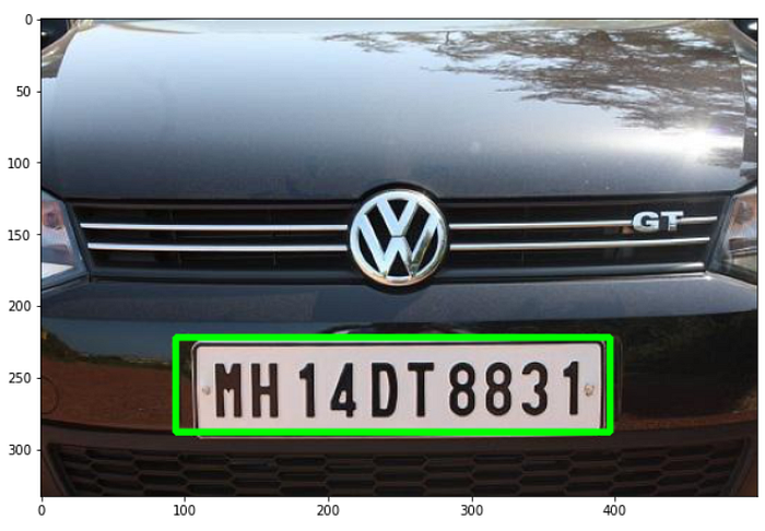

Predicted Box of Test Image

Fetching the Region of Interest (ROI) from the image using :

path='/test_images/N50.jpeg'
img=np.array(load_img(path))
xmin,xmax,ymin,ymax=coords[0]
roi=img[ymin:ymax,xmin:xmax]
plt.imshow(roi)
plt.show()

ROI of the Image

From this ROI piece we send it to Pytesseract function image_to_string.

As you can see it has extracted the Text from the License Plate.

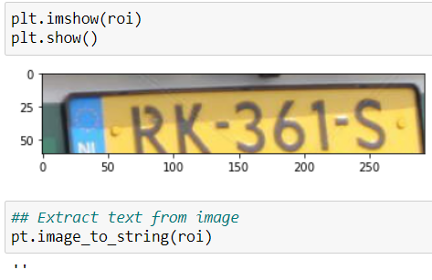
We see that this is a good scenario, but Pytesseract fails at number of places. For Example, in the below image it predicted well, but when the ROI is Provided to Pytesseract, it failed to read.

Failed to read a tilted image

Limitations of Pytesseract:

1. Pytesseract assumes that text is aligned in order, text should not be rotated or skewed
2. The Images should be very good and clean but not blurred.
3. Resolution of the image should be a min of 200 dpi or width and height should be atleast 300 pixels.
4. The Image should not be cropped.

So, I have went with another approach(YOLO), and this time it is much better than the Previously trained Model.

1. It has Improved precision on detecting License Plates.
2. Fast in Processing.

5 . Improving the Model using YOLO v5

YOLO, or You Only Look Once, is one of the most widely used deep learning based object detection algorithm.

Here, I will be training YOLO v5.

We will be following the below sequence of steps for the Training:

1. Yolo follows a format of having center_x, center_y, width, height using which the algorithm gets trained, so we will be building that.
2. Folder structure pattern of Train Images with its respective annotation files, and Test Images with its respective annotation files(txt format).
3. Data Preparation step for changing the format of annotation file from xml to text.
4. Creating YAML file, and cloning YOLO v5 repository, for training the data on Google Colab GPU for faster training.
5. Training the Model with YOLO.
6. Save the YOLO Model.
7. Interpreting the Model Results.

A. So firstly, we have the dataframe containing the information of all the Image files, its annotation, and respective information.

For YOLO Algorithm to work, we need to convert the existing data into the format suitable for it. It would need to have values for center_x, center_y, width and height as shown in figure below.

Basically, this is how it is represented for YOLO, as per image below.

defining height,width,center_x,center_y for YOLO

B. The Folder structure pattern should follow like the below figure. It needs to be segregated as per Train and Test Folders containing the image files and annotation files in txt format respectively.

Folder structure for YOLO — Train and Test

C. As far as data preparation step is concerned, we will be iterating through the xml files and extract the width and length for each of the file. Next we will be calculating the center_x, center_y using the code snippet below.

# parsing
def parsing(path):
    parser = xet.parse(path).getroot()
    name = parser.find('filename').text
    filename = f'./images/{name}'

    # width and height
    parser_size = parser.find('size')
    width = int(parser_size.find('width').text)
    height = int(parser_size.find('height').text)
    
    return filename, width, height
df[['filename','width','height']] = df['filepath'].apply(parsing).apply(pd.Series)

# center_x, center_y, width , height
df['center_x'] = (df['xmax'] + df['xmin'])/(2*df['width'])
df['center_y'] = (df['ymax'] + df['ymin'])/(2*df['height'])

df['bb_width'] = (df['xmax'] - df['xmin'])/df['width']
df['bb_height'] = (df['ymax'] - df['ymin'])/df['height']

Below is how it will be transformed to with the respective columns.

Next we will be building the code which helps in reading the dataframe data and copy the contents into a txt file with the respective columns like [width, height, center_x, center_y, bb_width, bb_height].

train_folder = './data_images/train'

values = df_train[['filename','center_x','center_y','bb_width','bb_height']].values
for fname, x,y, w, h in values:
    image_name = os.path.split(fname)[-1]
    txt_name = os.path.splitext(image_name)[0]
    
    dst_image_path = os.path.join(train_folder,image_name)
    dst_label_file = os.path.join(train_folder,txt_name+'.txt')
    
    # copy each image into the folder
    copy(fname,dst_image_path)

    # generate .txt which has label info
    label_txt = f'0 {x} {y} {w} {h}'
    with open(dst_label_file,mode='w') as f:
        f.write(label_txt)
        
        f.close()

upon transforming the data the file N100.txt, looks like in the below figure.

green boxes represent center_x, center_y, and blue boxes represent bb_width, bb_height.

Annotated as per YOLO format in txt format

D. For the purpose of training, we will be using Google Colab GPU, as it is faster.

We would need to prepare a yaml file with the paths for train and validation along with class information as shown below.

train: data_images/train
val: data_images/test
nc: 1
names: ['license_plate']

Open a Google Colab Notebook and perform the below steps.

Clone from the algorithm and its supporting files from the below URL.

!git clone https://github.com/ultralytics/yolov5

And then run the requirements.txt for installation in Google Colab.

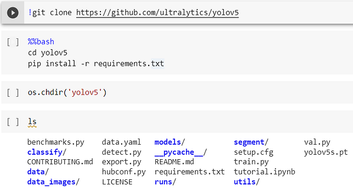
E. For training the Yolo Model, below is the command in colab for running 100 epochs.

!python train.py - data data.yaml - cfg yolov5s.yaml - batch-size 8 - name Model4 - epochs 100

Once the Model has run for 100 epochs, below the statistics and report.

We can see that YOLO v5 has 157 Layers, and Precision was 0.89 and Recall was 0.81

F. After the Model has ran, we will export the model weights for prediction needs.

!python export.py --weights runs/train/Model42/weights/best.pt --include onnx --simplify

G. We will export the folder and extract into our local to check the results of all the metrics which have being used.

6 . Metrics Evaluation

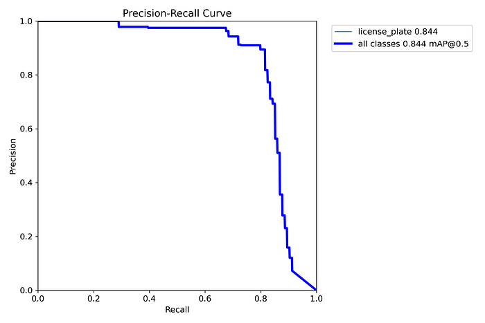
In our Model, we will focus on Precision — Recall curve.

The precision-recall curve shows the tradeoff between precision and recall for different threshold. A high area under the curve represents both high recall and high precision, where high precision relates to a low false positive rate, and high recall relates to a low false negative rate.

PR Curve

Lets have look at the True Labelled pictures, as shown in the figure and compare this with Predicted Images with License Plate detection.

License plate predictions with Probability

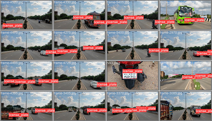
The above images properly detect the license plate and provides you with the probability as well.

7. Model Deployment and Execution using Flask App

As part of this case study, I have used Python Flask which helps in building Web Apps.

Following are the steps, I have taken to build the App.

1. Create app.py Python code importing the required Libraries, and the @app.route methods for the method invocation.
2. Created deeplearning.py for performing the activity of detecting the license plates, drawing rectangles around it, performing NMS(Non-Maximum Suppression), and extracting the text for display needs.

The code is available in GITHUB

8. Validating the model with Sample Demo and Test Images

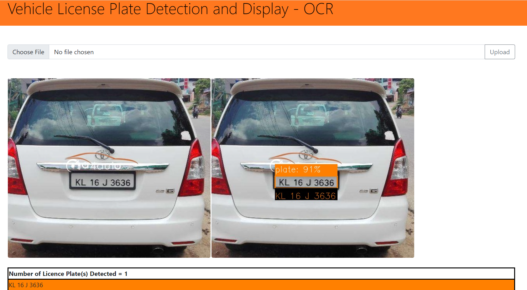
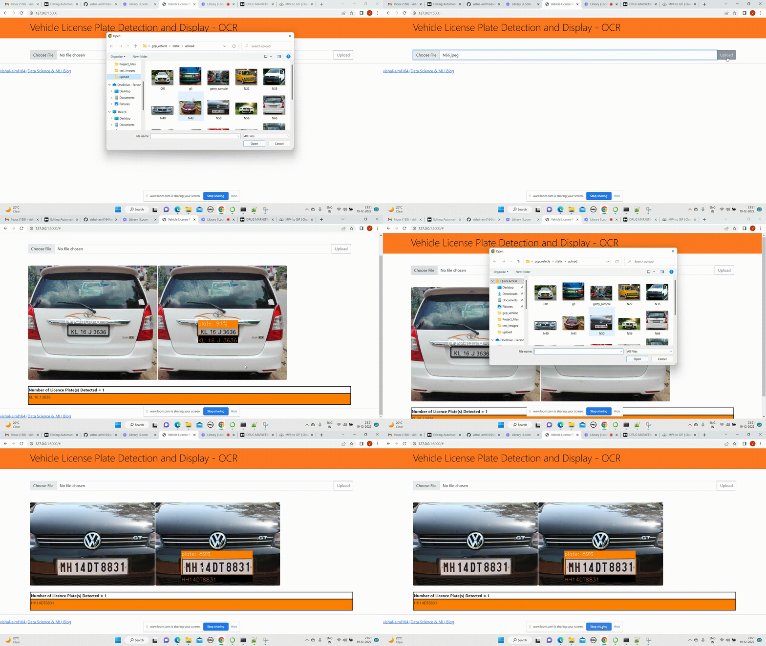
Here are sample Images after the Web App has being created.

As you can see left side image is the actual image, and right side is the one where the License plate is detected. In the below we are even able to see the extracted text displayed.

Next, lets take another example, as shown below.

Here is the full video of implementation using Flask App.(gif)

Here is the Full Video on Loom:

9. Future enhancements and References

1. For further improvements, we can collect more data and train much better models.
2. Upon getting more data, we could use different versions of YOLO v5, v7 etc.
3. We could even try with hough transformations, etc to ensure that even if plate is tilted, it would still give the result.

REFERENCES:

• www.appliedaicourse.com
• https://developer.nvidia.com/blog/creating-a-real-time-license-plate-detection-and-recognition-app/
• https://betterdatascience.com/detect-license-plates-with-yolo/
• https://github.com/heartexlabs/labelImg
• www.stackoverflow.com

The full code for this post can be found on Github. I look forward to hearing any feedback or comment.

Github Link : https://github.com/vishal-aiml164/vehicle-plate-v2

For few other case studies please refer below URL:

https://vishal-aiml164.github.io/vishal_aiml_portfolio/